How to read MSG SEVIRI data from the TROPOS archive?
This tutorial shows how to read MSG SEVIRI data at TROPOS using the MSevi data container class which is part of the python library collection tropy. The MSevi data container loads satellite data from hdf file if the hdf is available and the region is inside the predefined ‘eu’-domain. If not, then the MSevi class can also load the original HRIT files, but in this case no HRV input is implemented.
Import Libraries
[1]:
%matplotlib inline

# standard libs
import numpy as np
import datetime

# plotting and mapping
import pylab as plt
import cartopy.crs as ccrs
import cartopy.feature as cfeature
import seaborn as sns
sns.set_context('talk')

# the own tropy lib
from tropy.l15_msevi.msevi import MSevi
SEVIRI data are loaded into the MSevi data container.
Configuration of Rapid Scan
For configuration, we have to set region, scan_type and time (as object).
[2]:
time = datetime.datetime( 2013, 6, 8, 12, 0)
region = 'eu'
scan_type = 'rss'
Initialize the Data Container.
[3]:
s = MSevi(time = time, region = region, scan_type = scan_type)
Load Infrared Channel
Start with the infrared channel at 10.8 um.
[4]:
s.load('IR_108')
Region suggests use of hdf file
/vols/fs1/store/senf/.conda/python37/lib/python3.7/site-packages/h5py/_hl/dataset.py:313: H5pyDeprecationWarning: dataset.value has been deprecated. Use dataset[()] instead.
  "Use dataset[()] instead.", H5pyDeprecationWarning)
Now, the sat data are available as radiance (i.e. already converted from the counts using slope and offset). A dictionary s.rad is used to store the radiance information.
[5]:
print (s.rad)
{'IR_108': array([[ 53.30927581,  51.46395473,  48.59345526, ...,  77.29844993,
         78.32362831,  80.9890921 ],
       [ 55.56466825,  53.10424014,  47.15820553, ...,  79.14377102,
         80.78405643,  81.19412778],
       [ 52.89920446,  49.20856229,  41.41720659, ...,  72.58262938,
         76.6833429 ,  79.75887804],
       ...,
       [134.70843927, 136.55376035, 137.16886738, ...,  99.23726728,
         99.44230296,  99.44230296],
       [135.11851062, 135.11851062, 136.34872468, ...,  99.44230296,
         99.23726728,  99.44230296],
       [135.3235463 , 135.11851062, 135.73361765, ...,  99.44230296,
         99.23726728,  99.44230296]])}
What you want for infrared channel is perhaps the brightness temperature (BT). To get it, the is the method rad2bt that creates a BT dictionary under s.bt.
[6]:
s.rad2bt('IR_108')
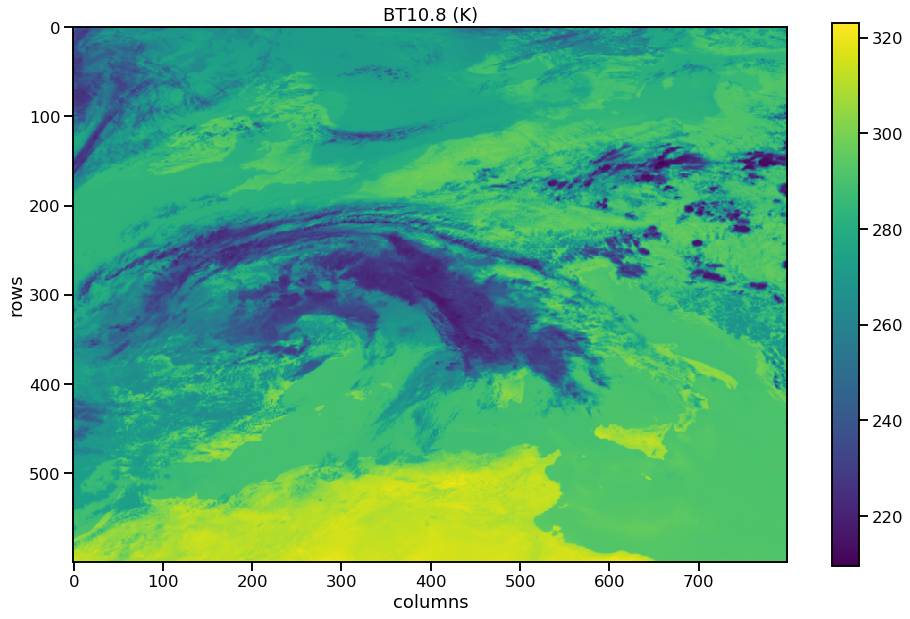
Plotting
[7]:
plt.figure( figsize = (16,10))
plt.imshow(s.bt['IR_108'])
plt.xlabel('columns')
plt.ylabel('rows')
plt.title('BT10.8 (K)')
plt.colorbar()
[7]:
<matplotlib.colorbar.Colorbar at 0x7f0f5f17b550>
Read the other Scan Type: Operational Scan
The SEVIRI operational scan is called pzs in our case. No hdf files are available, therefore the native HRIT format needs to be read.
[8]:
scan_type = 'pzs'
s = MSevi(time = time, region = 'eu', scan_type = scan_type)
s.load('IR_108')
s.rad2bt()
Region suggests use of hdf file
ERROR:  /vols/fs1/satellit/datasets/eumcst/msevi_pzs/l15_hdf/eu/2013/06/08/msg?-sevi-20130608t1200z-l15hdf-pzs-eu.c2.h5  does not exist!
... reading  /tmp/hrit4900095955/H-000-MSG3__-MSG3________-IR_108___-000007___-201306081200-__
... reading  /tmp/hrit4900095955/H-000-MSG3__-MSG3________-IR_108___-000008___-201306081200-__

Combine segments

Do calibration
Plotting
[9]:
plt.figure( figsize = (16,10))
plt.imshow(s.bt['IR_108'])
plt.xlabel('columns')
plt.ylabel('rows')
plt.title('BT10.8 (K)')
plt.colorbar()
[9]:
<matplotlib.colorbar.Colorbar at 0x7f0f5f086128>

It is slightly shifted! Do you see that?
Back to the Rapid Scan: Adjusting Region Configuration
[10]:
region = ((216, 456), (1676, 2076))
scan_type = 'rss'

s = MSevi(time = time, region = region, scan_type = scan_type)
[11]:
s.load('IR_108')
s.rad2bt('IR_108')
Region suggests use of hdf file
[12]:
plt.figure( figsize = (16,8))
plt.imshow(s.bt['IR_108'])
plt.xlabel('columns')
plt.ylabel('rows')
plt.title('BT10.8 (K)')
plt.colorbar()
[12]:
<matplotlib.colorbar.Colorbar at 0x7f0f5efbf630>

Getting geo-reference
The MSevi class also provides the method to read geo-reference, i.e. longitude and latitude (in deg), for the selected region cutout. The method is called s.lonlat() and the result is stored in the attributes s.lon and s.lat.
[13]:
s.lonlat()

print( s.lon, s.lat )
[[-0.3794155  -0.3231449  -0.26698685 ... 21.472942   21.529903
  21.58696   ]
 [-0.3580389  -0.30195236 -0.24592876 ... 21.446722   21.50356
  21.560478  ]
 [-0.33676338 -0.28081322 -0.22490978 ... 21.42049    21.47727
  21.53405   ]
 ...
 [ 2.335071    2.3752937   2.415495   ... 18.15725    18.197723
  18.238157  ]
 [ 2.3413725   2.3815722   2.421739   ... 18.149572   18.190002
  18.230433  ]
 [ 2.347673    2.3878417   2.427947   ... 18.141941   18.182312
  18.22275   ]] [[57.7341   57.731903 57.729946 ... 57.810207 57.81226  57.814465]
 [57.662613 57.660572 57.658646 ... 57.7384   57.740463 57.742657]
 [57.591175 57.58916  57.58723  ... 57.66635  57.668564 57.67074 ]
 ...
 [44.519314 44.518463 44.51767  ... 44.55012  44.551014 44.551758]
 [44.473633 44.47273  44.47193  ... 44.504284 44.505165 44.506012]
 [44.427914 44.42699  44.426296 ... 44.45857  44.459362 44.460358]]
Now, we plot again, but geo-referenced.
[14]:
plt.figure( figsize = (16,8))

ax = plt.axes(projection=ccrs.PlateCarree())
ax.coastlines( resolution='50m' )
ax.add_feature(cfeature.BORDERS, linestyle=':')

plt.pcolormesh(s.lon, s.lat, s.bt['IR_108'])
plt.title('BT10.8 (K)')
plt.colorbar()
[14]:
<matplotlib.colorbar.Colorbar at 0x7f0f5eedcd68>

Okay, this set of plotting methods might be needed. Let’s make a function:
Loading several channels
Now, we make a channel list and read all channels. The easied way is the get the default channel list from the msevi config.
[15]:
from tropy.l15_msevi.msevi_config import _narrow_channels
print( _narrow_channels )

full_channel_list = _narrow_channels + ['HRV',]
['VIS006', 'VIS008', 'IR_016', 'IR_039', 'WV_062', 'WV_073', 'IR_087', 'IR_097', 'IR_108', 'IR_120', 'IR_134']
[16]:
s.load(full_channel_list)
print( s.rad.keys())
Region suggests use of hdf file
dict_keys(['IR_108', 'VIS006', 'VIS008', 'IR_016', 'IR_039', 'WV_062', 'WV_073', 'IR_087', 'IR_097', 'IR_120', 'IR_134', 'HRV'])
Juchu! All channels are loaded!
Now, we convert all IR channel radiances to BTs. No arg means all…
[17]:
s.rad2bt()
print (s.bt.keys())
dict_keys(['IR_108', 'IR_039', 'IR_087', 'IR_097', 'IR_120', 'IR_134', 'WV_062', 'WV_073'])
Time to explore the content. We loop over all IR channels…
[18]:
for chan_name in s.bt.keys():
    plt.figure( figsize = (16,8))

    ax = plt.axes(projection=ccrs.PlateCarree())
    ax.coastlines( resolution='50m' )
    ax.add_feature(cfeature.BORDERS, linestyle=':')

    plt.pcolormesh(s.lon, s.lat, s.bt[chan_name])
    plt.colorbar()
    plt.title(chan_name)


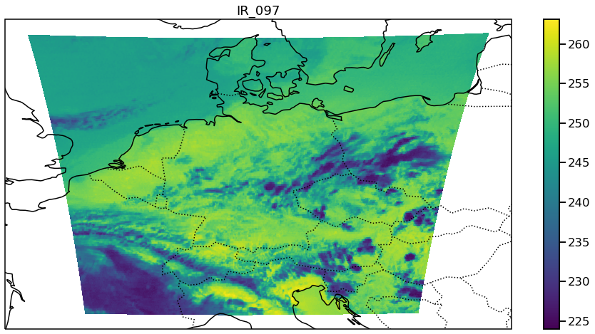


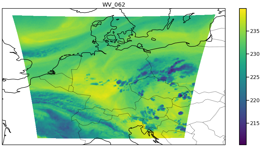

Wow, what a welth of information ;-)
But, visible is still missing, right? For this, there is the second conversion method called s.rad2refl that calculated reflectances. Note, no cos of solar zenith angle correction is applied here!
[19]:
s.rad2refl()
print (s.ref.keys())
dict_keys(['HRV', 'IR_016', 'VIS006', 'VIS008'])
Now, we plot the visible stuff.
First, the narrow-band channels.
[20]:
for chan_name in ['VIS006', 'VIS008', 'IR_016']:
    plt.figure( figsize = (16,8))

    ax = plt.axes(projection=ccrs.PlateCarree())
    ax.coastlines( resolution='50m' )
    ax.add_feature(cfeature.BORDERS, linestyle=':')

    plt.pcolormesh(s.lon, s.lat, s.ref[chan_name], cmap = plt.cm.gray)
    plt.colorbar()
    plt.title(chan_name)


Sat-Images are really beautiful!
HRV channel
We already loaded did all the input for HRV. We * loaded the radiances of the HRV channel * converted them to reflectances * and loaded georeference
With the narrow-band geo-ref, also a high-res geo-ref was calculated (just by linear interpolation). The high-res. lon and lat values are stored in the attributes s.hlon and s.hlat and can be used to plot and analyze HRV data
[21]:
plt.figure( figsize = (16,8))

ax = plt.axes(projection=ccrs.PlateCarree())
ax.coastlines( resolution='50m' )
ax.add_feature(cfeature.BORDERS, linestyle=':')

plt.pcolormesh(s.hlon, s.hlat, s.ref['HRV'], cmap = plt.cm.gray)
plt.colorbar()
plt.title('HRV')
[21]:
Text(0.5, 1.0, 'HRV')

Great detail in there!